Difference between revisions of "Data availability for the manuscript"
(→Model availability and reproduction of simulation results) |
(→Model availability and reproducibility of simulation results) |
||
| (10 intermediate revisions by the same user not shown) | |||
| Line 1: | Line 1: | ||
| − | ==Model availability and | + | ==Model availability and reproducibility of simulation results== |
| + | |||
| + | |||
===Access to the model=== | ===Access to the model=== | ||
| − | <p align=justify> The modular model with all submodules as well as values of the model parameters in each module are available on BioUML web-server online (click [https://sirius-web.org/bioumlweb/#de=data/Collaboration%20(git)/Muscle%20metabolism/Models/Integrated%20Model%202021/ here] and use "demo" access button) or can be accessed via | + | |
| + | <p align=justify> The modular model with all submodules as well as values of the model parameters in each module are available on <b>BioUML web-server online</b> (click [https://sirius-web.org/bioumlweb/#de=data/Collaboration%20(git)/Muscle%20metabolism/Models/Integrated%20Model%202021/ here] and use "demo" access button) or can be accessed via <b>GitLab</b> (click [https://gitlab.sirius-web.org/virtual-patient/muscle-metabolism here]). The model project is presented on the left side of the workspace:</p> | ||
| Line 8: | Line 11: | ||
{| align="center" style="background:#f8f9fa; border:1px solid #c8ccd1; font-size:100%; margin-center:1em" cellspacing=0 cellpadding=0 | {| align="center" style="background:#f8f9fa; border:1px solid #c8ccd1; font-size:100%; margin-center:1em" cellspacing=0 cellpadding=0 | ||
|- | |- | ||
| − | |<gallery mode="packed" heights=" | + | |<gallery mode="packed" heights="700px"> |
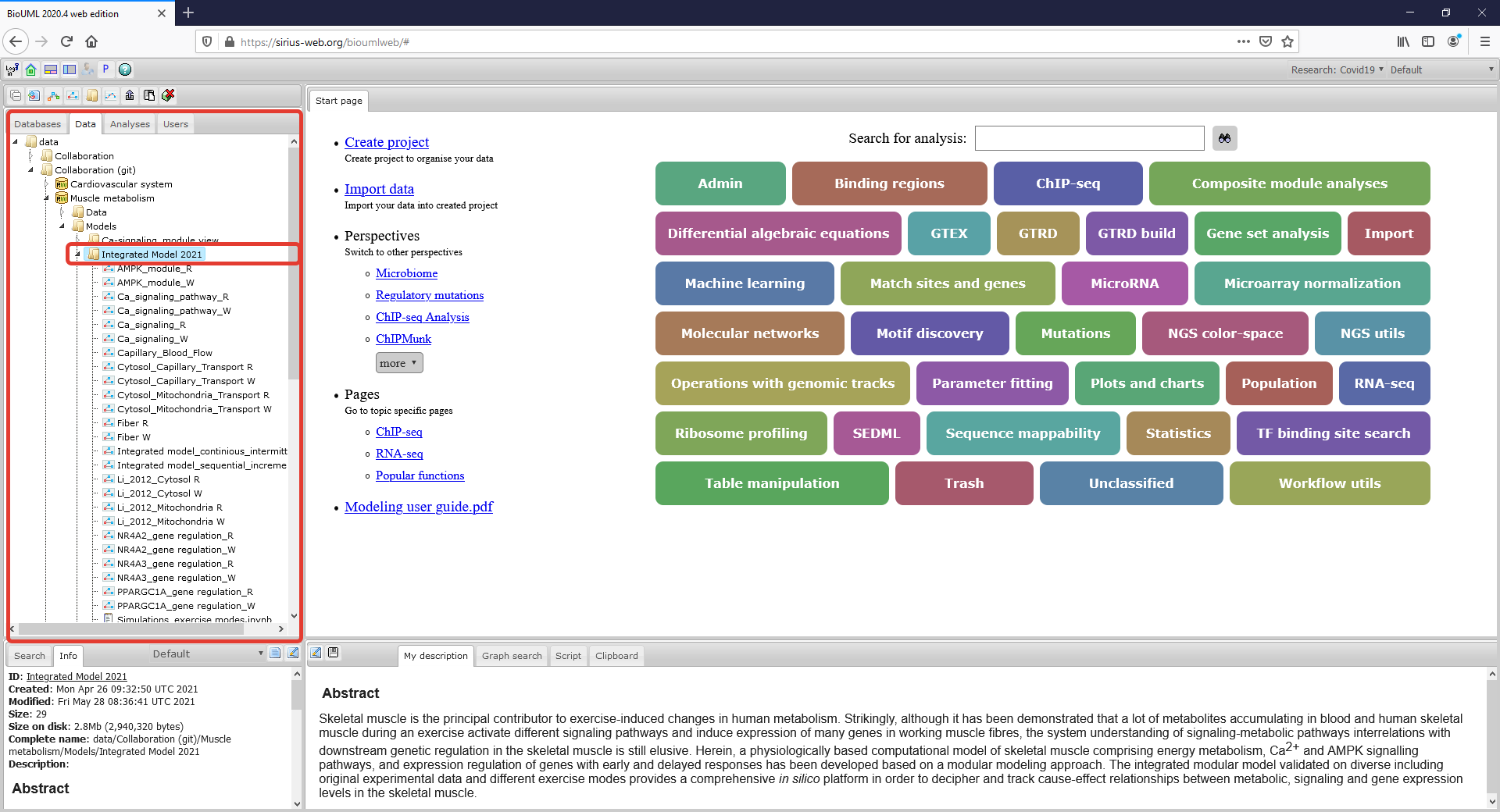
| − | Figure1_Project.png|<br><span style="font-size: 90%; align="right"">'''Figure 1.''' The workspace of the model project in web-version of the BioUML platform. Two rectangles with red borders indicate the | + | Figure1_Project.png|<br><span style="font-size: 90%; align="right"">'''Figure 1.''' The workspace of the model project in web-version of the BioUML platform. Two rectangles with red borders indicate the Tree area of the workspace and the corresponding place of the model project, respectively.</span> |
</gallery> | </gallery> | ||
|} | |} | ||
| Line 22: | Line 25: | ||
{| align="center" style="background:#f8f9fa; border:1px solid #c8ccd1; font-size:100%; margin-center:1em" cellspacing=0 cellpadding=0 | {| align="center" style="background:#f8f9fa; border:1px solid #c8ccd1; font-size:100%; margin-center:1em" cellspacing=0 cellpadding=0 | ||
|- | |- | ||
| − | |<gallery mode="packed" heights=" | + | |<gallery mode="packed" heights="700px"> |
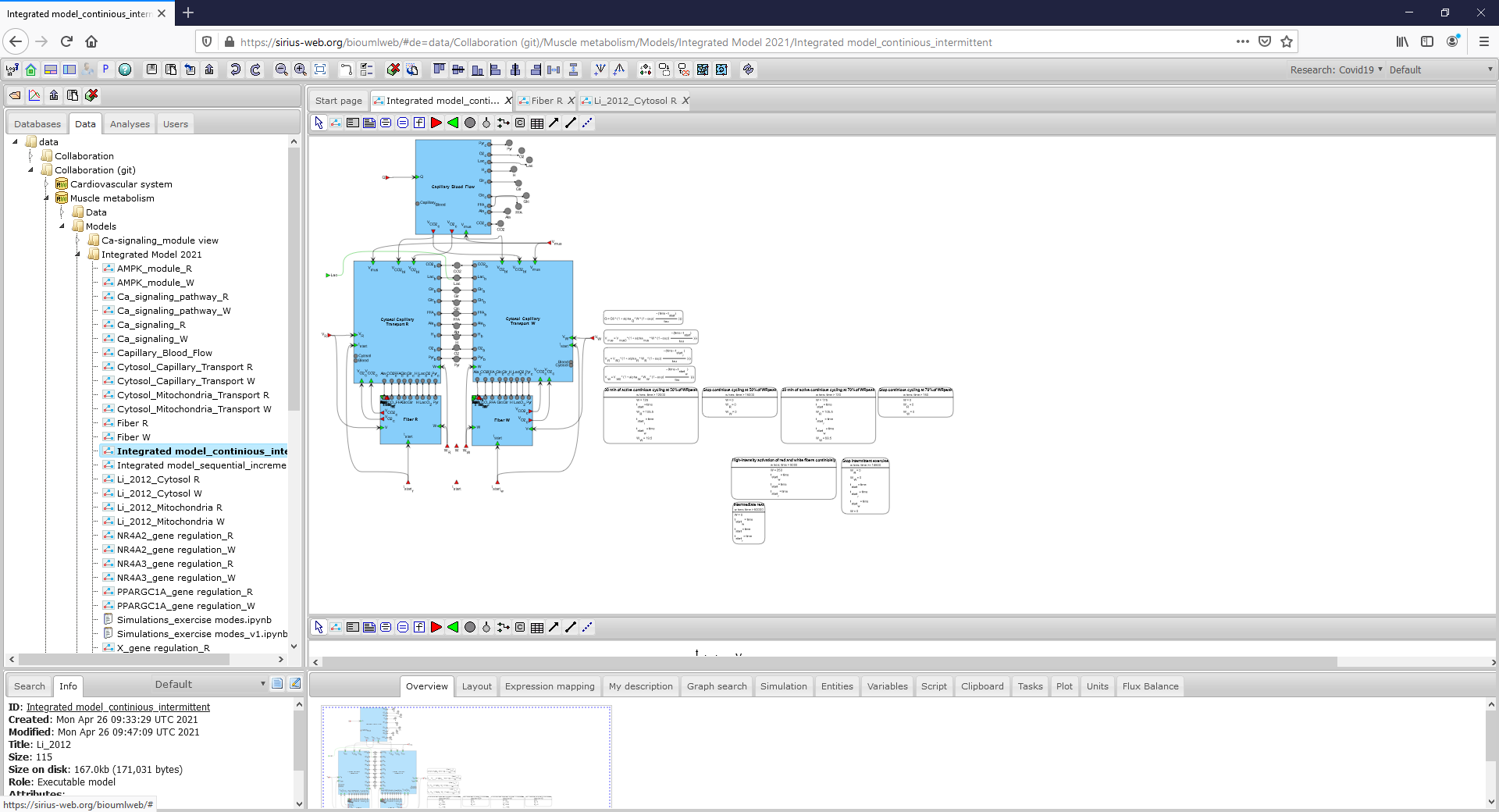
Figure2_Integrated_model.png|<br><span style="font-size: 90%; align="right"">'''Figure 2.1.''' An integrated modular model linking metabolism, Ca<sup>2+</sup>-dependent signaling transduction and regulation of gene expression in human skeletal muscle (To consider the model in more details click on the figure). </span> | Figure2_Integrated_model.png|<br><span style="font-size: 90%; align="right"">'''Figure 2.1.''' An integrated modular model linking metabolism, Ca<sup>2+</sup>-dependent signaling transduction and regulation of gene expression in human skeletal muscle (To consider the model in more details click on the figure). </span> | ||
| + | </gallery> | ||
| + | |} | ||
| + | {| align="center" style="background:#f8f9fa; border:1px solid #c8ccd1; font-size:100%; margin-center:1em" cellspacing=0 cellpadding=0 | ||
| + | |- | ||
| + | |<gallery mode="packed" heights="700px"> | ||
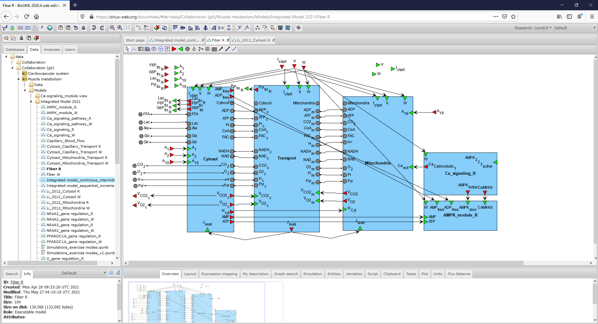
Figure2_FiberR.png|<br><span style="font-size: 90%; align="right"">'''Figure 2.2.''' A general SBGN diagram of the modular model describing metabolism in fibers I type taking into account metabolic processes in the cytoplasm, in the mitochondrion and transport reactions between two compartments (To consider the diagram in more details click on the figure). </span> | Figure2_FiberR.png|<br><span style="font-size: 90%; align="right"">'''Figure 2.2.''' A general SBGN diagram of the modular model describing metabolism in fibers I type taking into account metabolic processes in the cytoplasm, in the mitochondrion and transport reactions between two compartments (To consider the diagram in more details click on the figure). </span> | ||
</gallery> | </gallery> | ||
| Line 29: | Line 37: | ||
{| align="center" style="background:#f8f9fa; border:1px solid #c8ccd1; font-size:100%; margin-center:1em" cellspacing=0 cellpadding=0 | {| align="center" style="background:#f8f9fa; border:1px solid #c8ccd1; font-size:100%; margin-center:1em" cellspacing=0 cellpadding=0 | ||
|- | |- | ||
| − | |<gallery mode="packed" heights=" | + | |<gallery mode="packed" heights="700px"> |
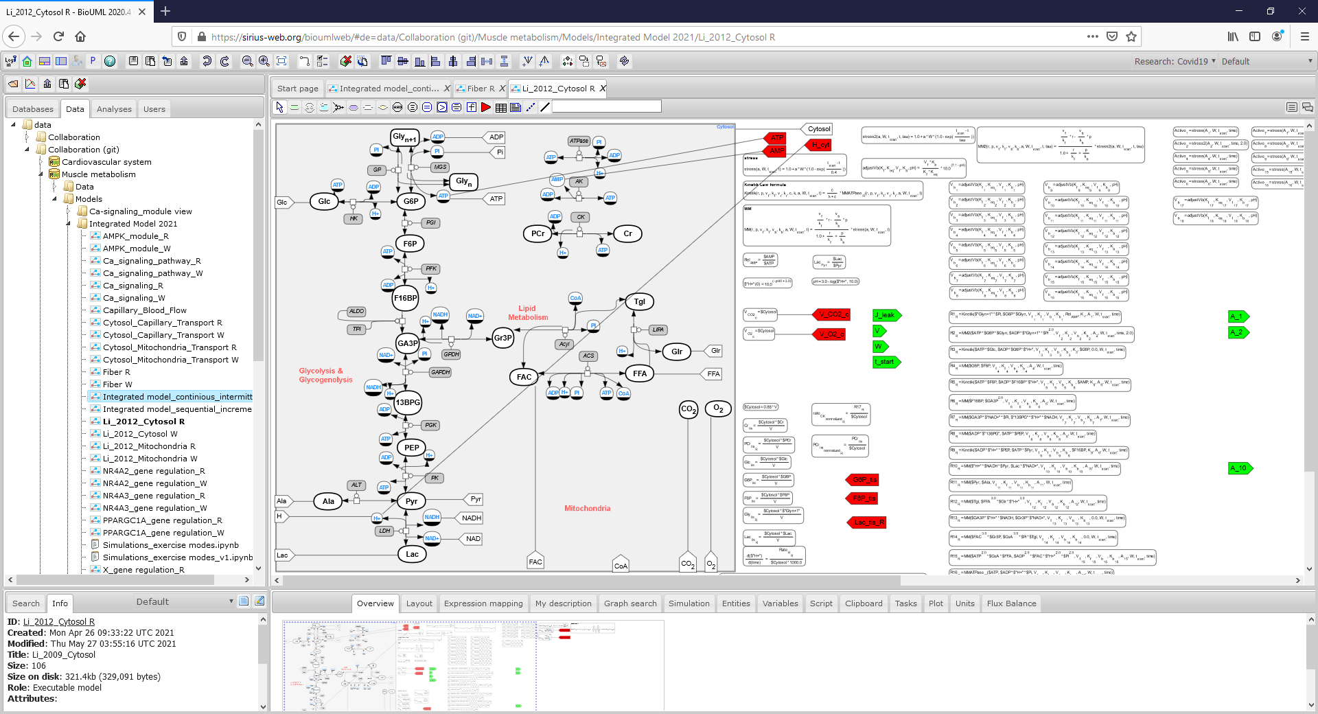
Figure2_CytosolR.png|<br><span style="font-size: 90%; align="right"">'''Figure 2.3.''' SBGN diagram of the cytosol compartment in fibers I type representing all metabolic reactions and corresponding math equations in the module.</span> | Figure2_CytosolR.png|<br><span style="font-size: 90%; align="right"">'''Figure 2.3.''' SBGN diagram of the cytosol compartment in fibers I type representing all metabolic reactions and corresponding math equations in the module.</span> | ||
| + | </gallery> | ||
| + | |} | ||
| + | |||
| + | |||
| + | |||
| + | <p align=justify> To consider or change the initial values of the model variables and parameter values click on the corresponding Menu Tab which is located below the diagram:</p> | ||
| + | |||
| + | |||
| + | |||
| + | {| align="center" style="background:#f8f9fa; border:1px solid #c8ccd1; font-size:100%; margin-center:1em" cellspacing=0 cellpadding=0 | ||
| + | |- | ||
| + | |<gallery mode="packed" heights="700px"> | ||
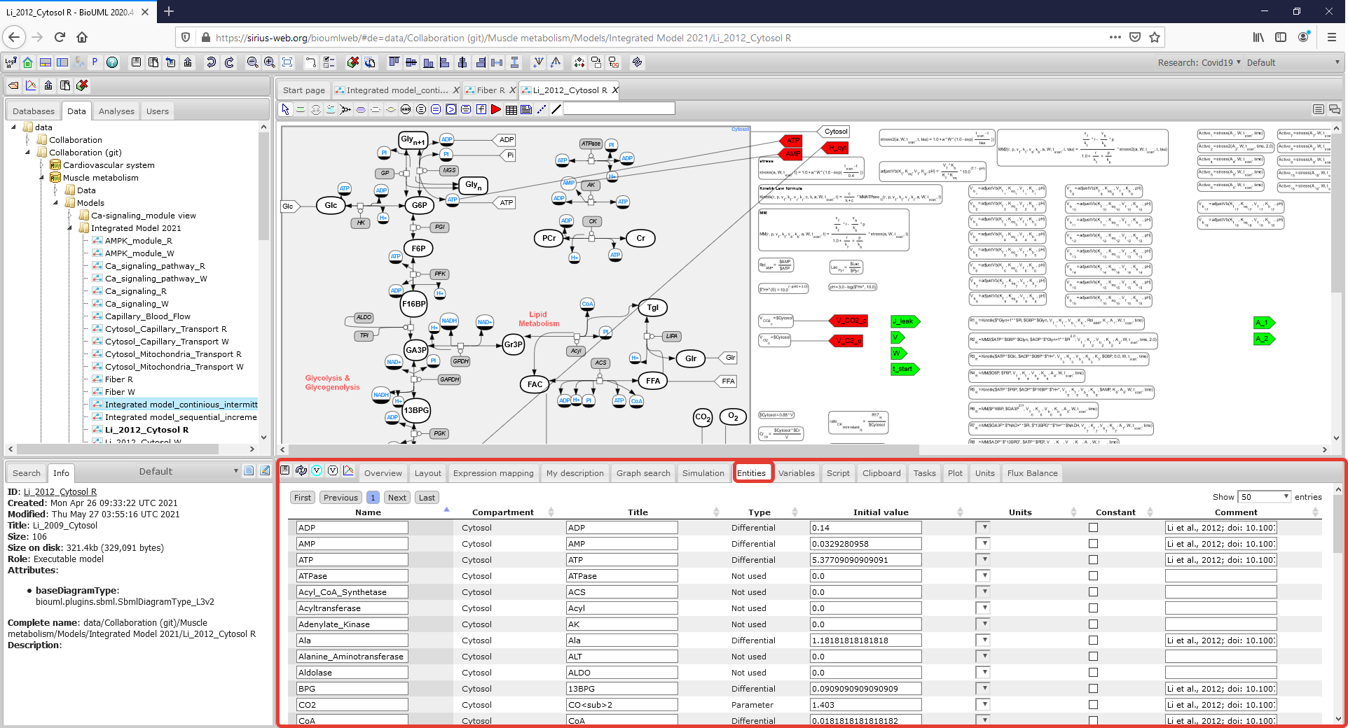
| + | Figure2_CytosolR_Entities.png|<br><span style="font-size: 90%; align="right"">'''Figure 3.1.''' A Menu Tab with initial values of the model variables is highlighted by a rectangle with a red border. (To consider the model in more details click on the figure). </span> | ||
| + | </gallery> | ||
| + | |} | ||
| + | {| align="center" style="background:#f8f9fa; border:1px solid #c8ccd1; font-size:100%; margin-center:1em" cellspacing=0 cellpadding=0 | ||
| + | |- | ||
| + | |<gallery mode="packed" heights="700px"> | ||
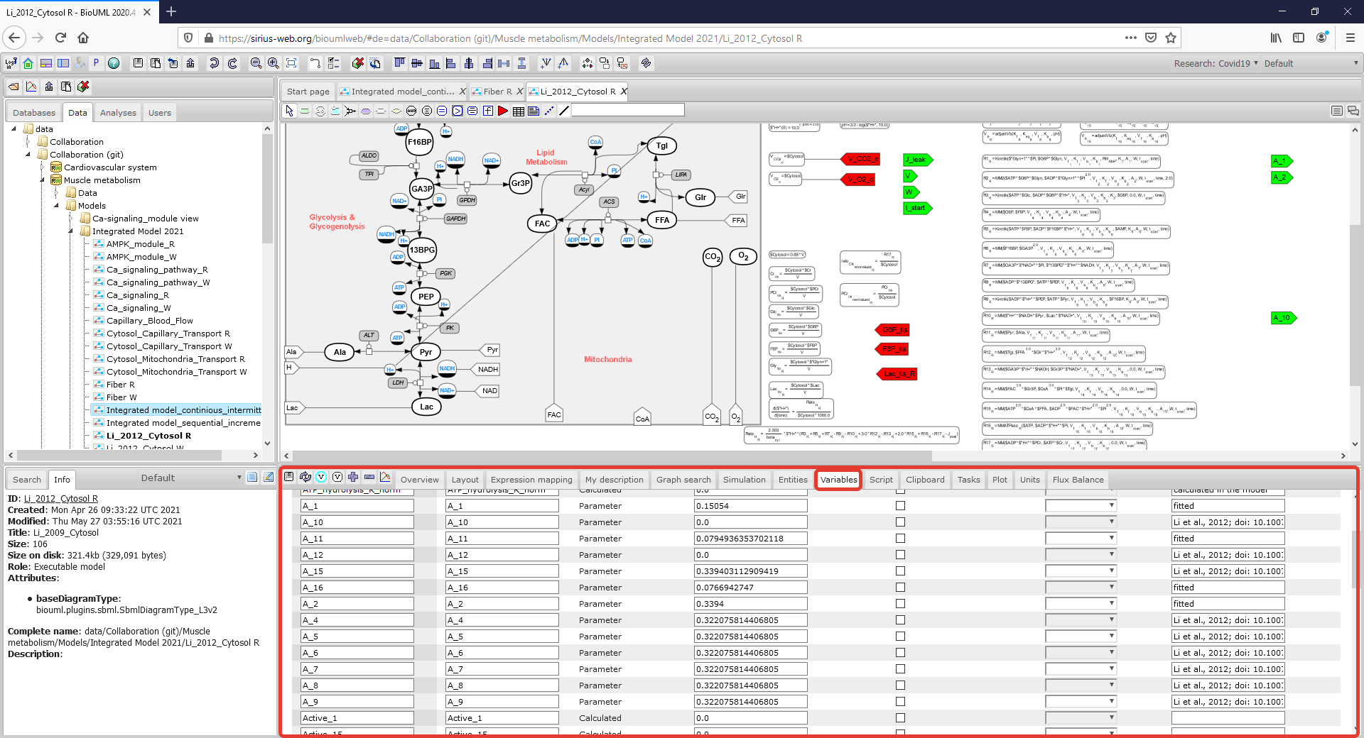
| + | Figure2_CytosolR_Variables.png|<br><span style="font-size: 90%; align="right"">'''Figure 3.2.''' A Menu Tab with parameter values of the model is highlighted by a rectangle with a red border. (To consider the model in more details click on the figure). </span> | ||
| + | </gallery> | ||
| + | |} | ||
| + | |||
| + | |||
| + | |||
| + | ===Simulate the model=== | ||
| + | |||
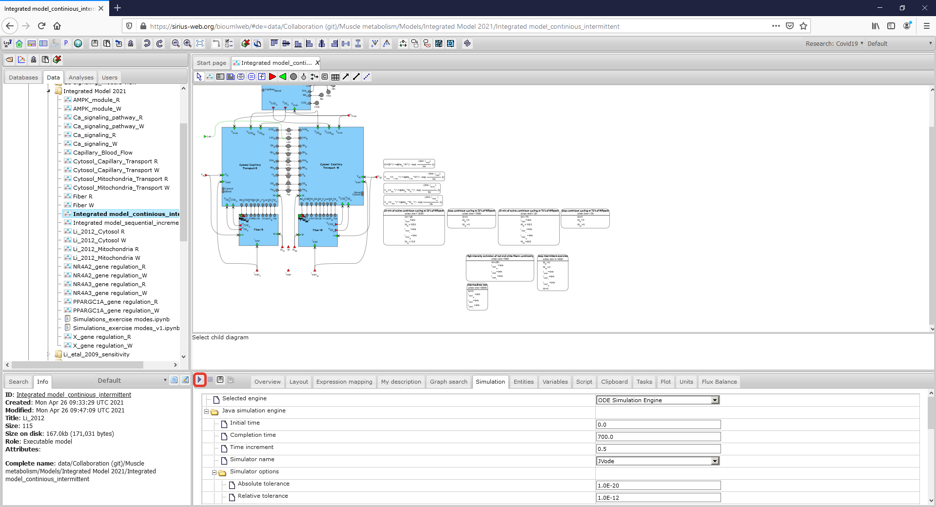
| + | <p align=justify> There are several ways to simulate the integrated model. The first one is to select the appropriate simulation engine clicking on <b><i> Simulation Tab </i></b> which is located below the diagram and push the <b><i> Simulation button</i></b> in this engine (in the rectangle with a red border):</p> | ||
| + | |||
| + | |||
| + | {| align="center" style="background:#f8f9fa; border:1px solid #c8ccd1; font-size:100%; margin-center:1em" cellspacing=0 cellpadding=0 | ||
| + | |- | ||
| + | |<gallery mode="packed" heights="700px"> | ||
| + | Figure3_Simulate.png|<br><span style="font-size: 90%; align="right"">'''Figure 4.''' To run the model employ Simulation tab. </span> | ||
| + | </gallery> | ||
| + | |} | ||
| + | |||
| + | |||
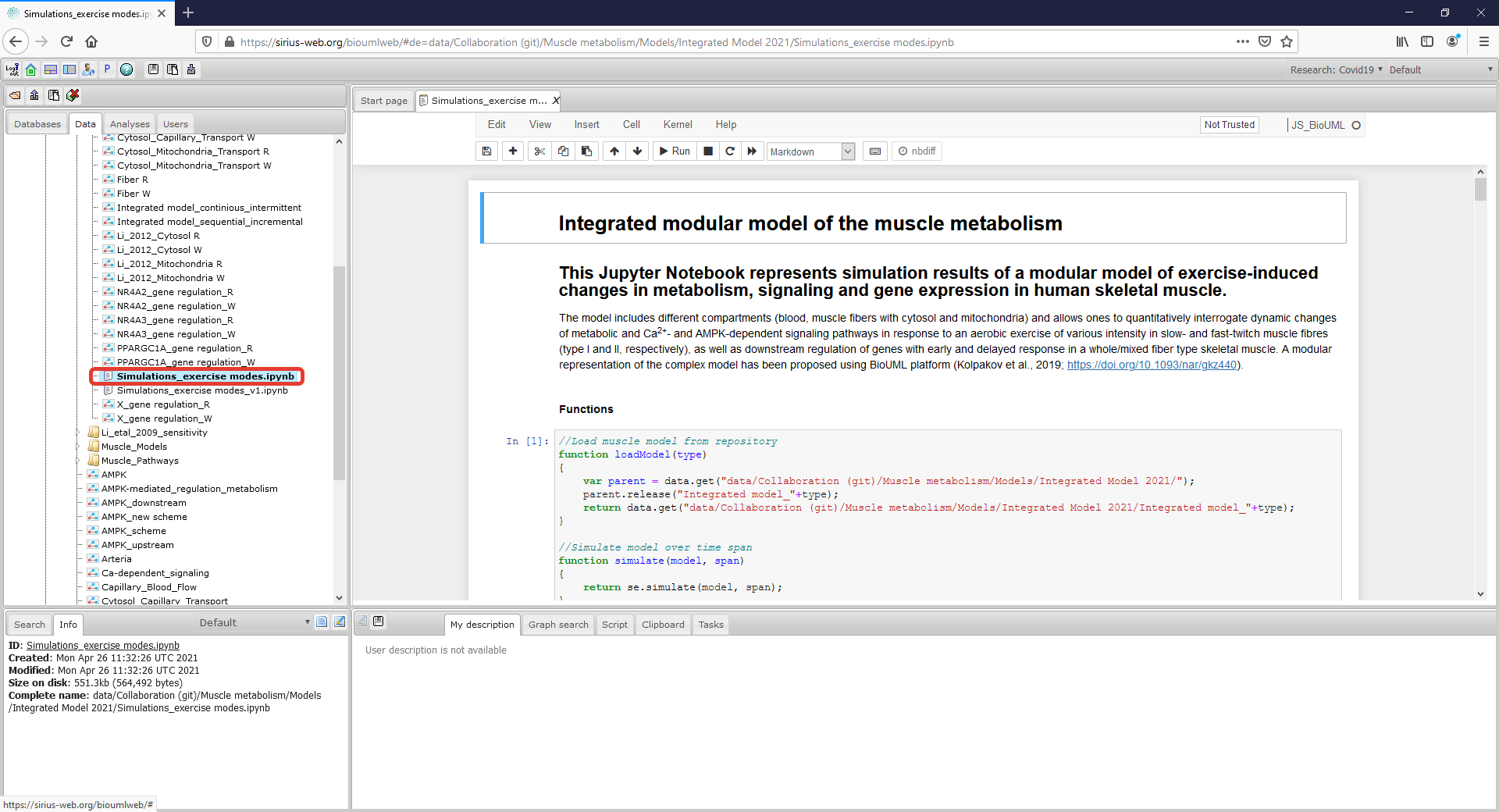
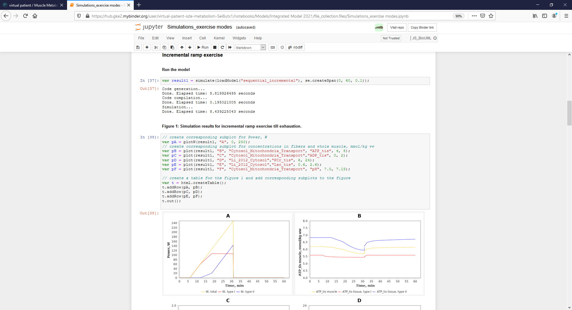
| + | <p align=justify> The second way to reproduce simulation results presented in the manuscript is to use created Jupyter Notebook (highlighted by a rectangle with a red border) in the Tree area of the model project (read-only mode for "demo" user) or launch the Notebook directly from GitLab using Binder web-service (registration is not required):</p> | ||
| + | |||
| + | |||
| + | |||
| + | {| align="center" style="background:#f8f9fa; border:1px solid #c8ccd1; font-size:100%; margin-center:1em" cellspacing=0 cellpadding=0 | ||
| + | |- | ||
| + | |<gallery mode="packed" heights="700px"> | ||
| + | Figure4_Simulate_Notebook.png|<br><span style="font-size: 90%; align="right"">'''Figure 5.1.''' Jupyter notebook provides reproducibility of results presented in the manuscript. The notebook can be started on the BioUML server - click on the corresponding ipynb file (highlighted by a rectangle with a red border). </span> | ||
| + | </gallery> | ||
| + | |} | ||
| + | {| align="center" style="background:#f8f9fa; border:1px solid #c8ccd1; font-size:100%; margin-center:1em" cellspacing=0 cellpadding=0 | ||
| + | |- | ||
| + | |<gallery mode="packed" heights="700px"> | ||
| + | Figure4_Simulate_Binder.png|<br><span style="font-size: 90%; align="right"">'''Figure 5.2.''' Jupyter notebook provides reproducibility of results presented in the manuscript. The notebook can be started via GitLab using Binder web-service - click on the corresponding launch icon (highlighted by a rectangle with a red border). </span> | ||
| + | </gallery> | ||
| + | |} | ||
| + | {| align="center" style="background:#f8f9fa; border:1px solid #c8ccd1; font-size:100%; margin-center:1em" cellspacing=0 cellpadding=0 | ||
| + | |- | ||
| + | |<gallery mode="packed" heights="700px"> | ||
| + | Figure4_Simulate_Binder_opened.png|<br><span style="font-size: 90%; align="right"">'''Figure 5.3.''' Binder allows a user to launch the Notebook in an executable environment.</span> | ||
</gallery> | </gallery> | ||
|} | |} | ||
Latest revision as of 15:55, 1 June 2021
Model availability and reproducibility of simulation results
Access to the model
The modular model with all submodules as well as values of the model parameters in each module are available on BioUML web-server online (click here and use "demo" access button) or can be accessed via GitLab (click here). The model project is presented on the left side of the workspace:
To open the integrated model or submodel diagram that is of interest, double click with the left mouse button on its icon in the Tree Area:
To consider or change the initial values of the model variables and parameter values click on the corresponding Menu Tab which is located below the diagram:
Simulate the model
There are several ways to simulate the integrated model. The first one is to select the appropriate simulation engine clicking on Simulation Tab which is located below the diagram and push the Simulation button in this engine (in the rectangle with a red border):
The second way to reproduce simulation results presented in the manuscript is to use created Jupyter Notebook (highlighted by a rectangle with a red border) in the Tree area of the model project (read-only mode for "demo" user) or launch the Notebook directly from GitLab using Binder web-service (registration is not required):
